KQUAD—A canonical kick quadrupole.

10.51 KQUAD—A canonical kick quadrupole.

A canonical kick quadrupole.
Parallel capable? : yes
GPU capable? : yes
Back-tracking capable? : yes


Parameter Name	Units	Type	Default	Description

L	M	double	0.0	length

K1	1∕M²	double	0.0	geometric strength

TILT	RAD	double	0.0	rotation about longitudinal axis

PITCH	RAD	double	0.0	rotation about horizontal axis. Ignored if MALIGN_METHOD=0

YAW	RAD	double	0.0	rotation about vertical axis. Ignored if MALIGN_METHOD=0.

BORE	M	double	0.0	bore radius

B	T	double	0.0	pole tip field (used if bore nonzero)

DX	M	double	0.0	misalignment

DY	M	double	0.0	misalignment

DZ	M	double	0.0	misalignment

FSE		double	0.0	fractional strength error

N_KICKS		long	0	number of kicks (rounded up to next multipole of 4 if INTEGRATION_ORDER=4). Deprecated. Use N_SLICES.

N_SLICES		long	1	Number of slices (full integrator steps).

HKICK	RAD	double	0.0	horizontal correction kick

VKICK	RAD	double	0.0	vertical correction kick

HCALIBRATION		double	1	calibration factor for horizontal correction kick

VCALIBRATION		double	1	calibration factor for vertical correction kick

HSTEERING		short	0	use for horizontal correction?

VSTEERING		short	0	use for vertical correction?

SYNCH_RAD		short	0	include classical, single-particle synchrotron radiation?

KQUAD continued

A canonical kick quadrupole.


Parameter Name	Units	Type	Default	Description

SYSTEMATIC_MULTIPOLES		STRING	NULL	input file for systematic multipoles

EDGE_MULTIPOLES		STRING	NULL	input file for systematic edge multipoles

RANDOM_MULTIPOLES		STRING	NULL	input file for random multipoles

STEERING_MULTIPOLES		STRING	NULL	input file for multipole content of steering kicks

SYSTEMATIC_MULTIPOLE_FACTOR		double	1	Factor by which to multiply systematic and edge multipoles

RANDOM_MULTIPOLE_FACTOR		double	1	Factor by which to multiply random multipoles

STEERING_MULTIPOLE_FACTOR		double	1	Factor by which to multiply steering multipoles

MIN_NORMAL_ORDER		short	-1	If nonnegative, minimum order of systematic and random normal multipoles to use from data files.

MIN_SKEW_ORDER		short	-1	If nonnegative, minimum order of systematic and random skew multipoles to use from data files.

MAX_NORMAL_ORDER		short	-1	If nonnegative, maximum order of systematic and random normal multipoles to use from data files.

MAX_SKEW_ORDER		short	-1	If nonnegative, maximum order of systematic and random skew multipoles to use from data files.

INTEGRATION_ORDER		short	4	integration order (2, 4, or 6)

SQRT_ORDER		short	0	Ignored, kept for backward compatibility only.

ISR		short	0	include incoherent synchrotron radiation (quantum excitation)?

KQUAD continued

A canonical kick quadrupole.


Parameter Name	Units	Type	Default	Description

ISR1PART		short	1	Include ISR for single-particle beam only if ISR=1 and ISR1PART=1

SR_IN_ORDINARY_MATRIX		short	0	If nonzero, the (tracking-based) matrix used for routine computations includes classical synchrotron radiation if SYNCH_RAD=1.

EDGE1_EFFECTS		short	0	include entrance edge effects?

EDGE2_EFFECTS		short	0	include exit edge effects?

LEFFECTIVE	M	double	0.0	Effective length. Ignored if non-positive.

I0P	M	double	0.0	i0+ fringe integral

I1P	M²	double	0.0	i1+ fringe integral

I2P	M³	double	0.0	i2+ fringe integral

I3P	M⁴	double	0.0	i3+ fringe integral

LAMBDA2P	M³	double	0.0	lambda2+ fringe integral

I0M	M	double	0.0	i0- fringe integral

I1M	M²	double	0.0	i1- fringe integral

I2M	M³	double	0.0	i2- fringe integral

I3M	M⁴	double	0.0	i3- fringe integral

LAMBDA2M	M³	double	0.0	lambda2- fringe integral

EDGE1_LINEAR		short	1	Use to selectively turn off linear part if EDGE1_EFFECTS nonzero.

EDGE2_LINEAR		short	1	Use to selectively turn off linear part if EDGE2_EFFECTS nonzero.

EDGE1_NONLINEAR_FACTOR		double	1	Use to selectively scale nonlinear entrance edge effects if EDGE1_EFFECTS>1

EDGE2_NONLINEAR_FACTOR		double	1	Use to selectively scale nonlinear exit edge effects if EDGE2_EFFECTS>1

RADIAL		short	0	If non-zero, converts the quadrupole into a radially-focusing lens

KQUAD continued

A canonical kick quadrupole.


Parameter Name	Units	Type	Default	Description

EXPAND_HAMILTONIAN		short	0	If 1, Hamiltonian is expanded to leading order.

TRACKING_MATRIX		short	0	If nonzero, gives order of tracking-based matrix up to third order to be used for twiss parameters etc. If zero, 2nd-order analytical matrix is used.

MALIGN_METHOD		short	0	0=original, 1=new entrace-centered, 2=new body-centered

GROUP		string	NULL	Optionally used to assign an element to a group, with a user-defined name. Group names will appear in the parameter output file in the column ElementGroup

This element simulates a quadrupole using a kick method based on symplectic integration. The user specifies the number of kicks and the order of the integration. For computation of twiss parameters and response matrices, this element is treated like a standard thick-lens quadrupole; i.e., the number of kicks and the integration order become irrelevant.

Multipole errors

Specification of systematic and random multipole errors is supported through the SYSTEMATIC_MULTIPOLES, EDGE_MULTIPOLES, and RANDOM_MULTIPOLES fields. These specify, respectively, fixed multipole strengths for the body of the element, fixed multipole strengths for the edges of the element, and random multipole strengths for the body of the element. These fields give the names of SDDS files that supply the multipole data. The files are expected to contain a single page of data with the following elements:

Floating point parameter referenceRadius giving the reference radius for the multipole data.
An integer column named order giving the order of the multipole. The order is defined as (N_poles - 2)∕2, so a quadrupole has order 1, a sextupole has order 2, and so on.
Floating point columns normal and skew giving the values for the normal and skew multipole strengths, respectively. (N.B.: previous versions used the names an and bn, respectively. This is still accepted but deprecated) These are defined as a fraction of the main field strength measured at the reference radius, R: f_n = , where m = 1 is the order of the main field and n is the order of the error multipole. A similar relationship holds for the skew multipole fractional strengths. For random multipoles, the values are interpreted as rms values for the distribution.

Specification of systematic higher multipoles due to steering fields is supported through the STEERING_MULTIPOLES field. This field gives the name of an SDDS file that supplies the multipole data. The file is expected to contain a single page of data with the following elements:

Floating point parameter referenceRadius giving the reference radius for the multipole data.
An integer column named order giving the order of the multipole. The order is defined as (N_poles - 2)∕2. The order must be an even number because of the quadrupole symmetry.
Floating point column normal giving the values for the normal multipole strengths, which are driven by the horizontal steering field. (N.B.: previous versions used the name an for this data. This is still accepted but deprecated) normal is specifies the multipole strength as a fraction f_n of the steering field strength measured at the reference radius, R: f_n = , where m = 0 is the order of the steering field and n is the order of the error multipole. The skew values (for vertical steering) are deduced from the normal values, specifically, g_n = f_n * (-1)^n∕2.

The dominant systematic multipole term in the steering field is a sextupole. Note that elegant presently does not include such sextupole contributions in the computation of the chromaticity via the twiss_output command. However, these chromatic effects will be seen in tracking.

Apertures

Apertures specified via an upstream MAXAMP element or an aperture_input command will be imposed inside this element.

Length specificiation

As of version 29.2, this element incorporates the ability to have different values for the insertion and effective lengths. This is invoked when LEFFECTIVE is positive. In this case, the L parameter is understood to be the physical insertion length. Using LEFFECTIVE is a convenient way to incorporate the fact that the effective length may differ from the physical length and even vary with excitation, without having to modify the drift spaces on either side of the quadrupole element.

Fringe effects

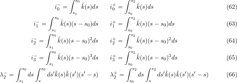
Fringe field effects are based on publications of D. Zhuo et al. [34] and J. Irwin et al. [35], as well as unpublished work of C. X. Wang (ANL). The fringe field is characterized by 10 integrals given in equations 19, 20, and 21 of [34]. However, the values input into elegant should be normalized by K₁ or K₁², as appropriate.

For the exit-side fringe field, let s₁ be the center of the magnet, s₀ be the location of the nominal end of the magnet (for a hard-edge model), and let s₂ be a point well outside the magnet. Using K_1,he(s) to represent the hard edge model and K₁(s) the actual field profile, we define the normalized difference as (s) = (K₁(s) - K_1,he(s))∕K₁(s₁). (Thus, (s) = (s)∕K₀, using the notation of Zhou et al.)

The integrals to be input to elegant are defined as

∫ s0 ∫ s2 i-0 = ˜k(s)ds i+0 = ˜k (s)ds (62) ∫ s1 ∫s0 - s0˜ + s2˜ i1 = s1 k(s)(s - s0)ds i1 = s0 k (s)(s- s0)ds (63) ∫ s0 ∫ s2 i-2 = ˜k(s)(s - s0)2ds i+2 = ˜k (s)(s- s0)2ds (64) ∫s1 ∫s0 - s0˜ 3 + s2˜ 3 i3 = s k(s)(s - s0) ds i3 = s k (s)(s- s0) ds (65) ∫ s0 ∫ s0 1 ∫0s2 ∫ s2 λ -2 = ds ds′˜k(s)˜k(s′)(s′ - s) λ+2 = ds ds′˜k(s)˜k(s′)(s′ - s) (66) s1 s s0 s

Normally, the effects are dominated by i₁^- and i₁⁺. The script computeQuadFringeIntegrals, packaged with elegant, allows computing these integrals and the effective length if provided with data giving the gradient vs s.

The EDGE1_EFFECTS and EDGE2_EFFECTS parameters can be used to turn fringe field effects on and off, but also to control the order of the implementation. If the value is 1, linear fringe effects are included. If the value is 2, leading-order (cubic) nonlinear effects are included. If the value is 3 or higher, higher order effects are included.

Misalignments

There are three modes for implementing alignment errors. Which is used is controlled by the value of the MALIGN_METHOD parameter:

MALIGN_METHOD=0 — This selects the original method, which was the only one available before version 2021.1. The misalignment is referenced to the entrance face. The YAW and PITCH parameters are ignored.
MALIGN_METHOD=1 — This selects a linearized method based on M. Venturini’s work [58], with misalignment referenced to the entrance face. The YAW and PITCH parameters are implemented.
MALIGN_METHOD=2 — This selects a linearized method based on M. Venturini’s work [58], with misalignment referenced to the magnet center. The YAW and PITCH parameters are implemented.
MALIGN_METHOD=3 — This selects an exact method based on M. Venturini’s work [58], with misalignment referenced to the entrance face. The YAW and PITCH parameters are implemented.
MALIGN_METHOD=4 — This selects an exact method based on M. Venturini’s work [58], with misalignment referenced to the magnet center. The YAW and PITCH parameters are implemented.

For elements with non-zero TILT, error displacements and rotations are performed in the lab frame.

Radiation effects

If SYNCH_RAD is non-zero, classical synchrotron radiation is included in tracking. If, in addition, ISR is non-zero, incoherent synchrotron radiation (i.e., quantum-mechanical variation in radiation emitted by different particles) is also included. (To exclude ISR for single-particle tracking, set ISR1PART=0.)

If TRACKING_MATRIX and SYNCH_RAD are non-zero, classical synchrotron radiation can be included in the ordinary matrix (e.g., for twiss_output and matrix_output) by setting SR_IN_ORDINARY_MATRIX to a non-zero value. Symplecticity is not assured, but the results may be interesting nonetheless. A more rigorous approach is to use moments_output. SR_IN_ORDINARY_MATRIX does not affect tracking.

KQUSE

[next] [prev] [prev-tail] [front] [up]